Joint Distribution of Discrete and Continuous Random Variables

The joint distribution function is a function that completely characterizes the probability distribution of a random vector.

Table of contents

1. Synonyms and acronyms

2. Joint cdf of X and Y

3. Example

4. The formula for discrete variables

5. How to compute the formula with a table

6. The formula for continuous variables

   1. Example

7. How to derive the marginal cdfs from the joint

8. Deriving the joint cdf from the marginals

9. Joint cdf of two independent variables

10. A more general definition

11. More details

12. Keep reading the glossary

It is also called joint cumulative distribution function (abbreviated as joint cdf).

Let us start with the simple case in which we have two random variables and .

Their joint cdf is defined as where and are two real numbers.

Note that:

• indicates a probability;

• the comma inside the parentheses stands for AND.

In other words, the joint cdf gives the probability that two conditions are simultaneously true:

• the random variable takes a value less than or equal to ;

• the random variable takes a value less than or equal to .

Suppose that there are only four possible cases:

Further assume that each of these cases has probability equal to 1/4.

Let us compute, as an example, the following value of the joint distribution function:

The two conditions that need to be simultaneously true are:

There are two cases in which they are satisfied:

Therefore, we have

In the previous example we have shown a special case.

In general, the formula for the joint cdf of two discrete random variables and is: where:

The probabilities in the sum are often written using the so-called joint probability mass function

The sum in the formula above can be easily computed with the help of a table.

Here is an example.

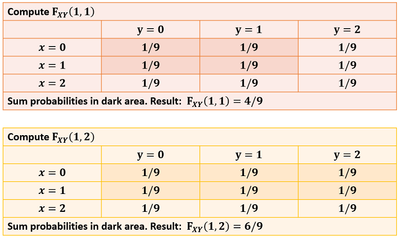
In this table, there are nine possible couples and they all have the same probability (1/9).

In order to compute the joint cumulative distribution function, all we need to do is to shade all the probabilities to the left of (included) and above (included).

Then, the value of is equal to the sum of the probabilities in the shaded area.

When and are continuous random variables, we need to use the formula where is the joint probability density function of and .

The computation of the double integral can be broken down in two steps:

1. first compute the inner integral which, in general, is a function of and ;

2. then calculate the outer integral

Example

Let us make an example.

Let the joint pdf be

When and , we have

This is only one of the possible cases. We also have the two cases:

1. or , in which case

2. and , in which case

The two marginal distribution functions of and are

They can be derived from the joint cumulative distribution function as follows: where the exact meaning of the notation is

This can be demonstrated as follows: because the condition is always met and, as a consequence, the condition is satisfied whenever is true.

The proof for is analogous.

In general, we cannot derive the joint cdf from the marginals, unless we know the so-called copula function, which links the two marginals.

However, there is an important exception, discussed in the next section.

When and are independent, then the joint cdf is equal to the product of the marginals:

See the lecture on independent random variables for a proof, a discussion and some examples.

Until now, we have discussed the case of two random variables. However, the joint cdf is defined for any collection of random variables forming a random vector.

Definition The joint distribution function of a random vector is a function such that: where the entries of and are denoted by and respectively, for .

More details about joint distribution functions can be found in the lecture entitled Random vectors.

Previous entry: Integrable random variable

Next entry: Joint probability density function

Please cite as:

Taboga, Marco (2021). "Joint distribution function", Lectures on probability theory and mathematical statistics. Kindle Direct Publishing. Online appendix. https://www.statlect.com/glossary/joint-distribution-function.

quintanasurew1950.blogspot.com

Source: https://statlect.com/glossary/joint-distribution-function

Share this post